A Beginner's Guide to Linear Regression: Understanding the Fundamentals

Introduction to Linear Regression

Linear regression is one of the simplest and most widely used techniques in statistics and machine learning. It is a foundational concept that helps us understand the relationships between variables, making it a crucial tool in predictive modeling.

What is Linear Regression?

Linear regression is a supervised learning algorithm used for predicting a continuous target variable based on one or more input features. The goal is to model the relationship between the dependent variable (target) and independent variable(s) (predictors) using a straight line.

Linear regression is a method for modeling the relationship between one dependent variable (the outcome or target) and one or more independent variables (predictors or features). The objective is to fit a straight line (in the simplest case) through a dataset that best represents this relationship.

‍

• In simple linear regression, we study the relationship between a single predictor and the target.
• In multiple linear regression, multiple predictors are used to predict the target.

Linear regression assumes that changes in the predictors correspond to proportional changes in the target variable, forming a linear relationship.

Also read:How to Learn Machine Learning

‍

Example:
Imagine you are a business analyst trying to predict a company's future revenue based on its advertising spending. Linear regression can help determine how advertising impacts revenue and predict future values.

Why Use Linear Regression?

Linear regression offers several advantages:

1. Ease of Use: Its simplicity makes it a great starting point for beginners.
2. Interpretability: The model parameters (coefficients) explain the magnitude and direction of the relationship between variables.
3. Broad Applicability: Linear regression can be used in diverse fields like economics, biology, engineering, and beyond.

‍

Importance of Linear Regression

1. Modeling Relationships:
   Linear regression helps answer questions like:some text
   • "Does spending more on marketing lead to higher sales?"
   • "How does temperature affect ice cream sales?"
2. Predictive Analysis:
   Once a relationship is established, linear regression can predict outcomes based on new data.
3. Feature Selection:
   By analyzing the coefficients, linear regression provides insights into which predictors are the most influential.
4. Foundation for Complex Models:
   It serves as a gateway to advanced machine learning techniques, such as logistic regression, polynomial regression, and neural networks.

‍

Real-World Applications of Linear Regression

• Finance: Predicting stock prices or market trends.
• Healthcare: Estimating patient recovery times based on treatment factors.
• Marketing: Assessing the effect of advertising campaigns on sales.
• Agriculture: Forecasting crop yield based on rainfall and temperature.

Suppose you are a student trying to predict your exam score based on study hours. You observe that studying more hours generally leads to higher scores. Linear regression helps quantify this relationship, enabling you to predict a likely score for, say, 5 hours of study.

‍

The Linear Regression Equation

Linear regression revolves around a simple but powerful mathematical equation that represents the relationship between the dependent variable (Y) and the independent variable(s) (X).

The General Form of the Linear Regression Equation

Linear regression equations can be represented using different notations depending on the context or discipline. Let’s explore the most commonly used notations:

The notation (fw,b( X)=wX+b) is a concise way of representing the linear regression hypothesis function often seen in machine learning contexts. Let's break it down:

Components of (fw,b( X)=wX+b) :

1. fw,b( X):some text
   • This represents the hypothesis function. It takes the input x and maps it to the predicted output based on the parameters w and b.
   • The subscript w,b emphasizes that the prediction depends on the parameters w (weights) and b (bias).
2.   w:some text
   • Known as the weight, it determines the slope of the line (or the magnitude of the effect of X on Y).
   • In higher dimensions (multiple features), w becomes a vector of weights.
3. x:some text
   • The input feature(s) (independent variable(s)).
   • For a single feature, x is a scalar. For multiple features, x  is a vector, and wx represents a dot product.
4. b:some text
   • The bias or intercept term. It adjusts the model to fit the data when X=0.

Intuitive Interpretation

• w controls how steeply Y changes with X.some text
  • Larger w: A steeper slope.
  • Smaller w: A flatter slope.
• b shifts the entire line up or down without changing its slope.

For instance:

• If w=2 and b=3, the equation becomes:  fw,b( X)=2X+3 . The line has a slope of 2 and an intercept at Y=3.

‍

Extension to Multivariable Linear Regression

For multiple features, X becomes a vector X=[X1​,X2​,…,Xn​] , and w becomes a corresponding vector of weights w=[w1,w2,…,wn]. The equation is:

Where w⋅X is the dot product of the weights and features.

The equation (fw,b( X)=wX+b) represents a line in 2D space for single-variable regression.

In higher dimensions, it represents a hyperplane where w defines the orientation, and b determines its position relative to the origin.

Assumptions of Linear Regression

1. Linearity: The relationship between the independent variables and the dependent variable is linear. Non-linear trends can lead to inaccurate predictions.
   
   
2. Independence of Errors: The residuals (errors) are independent of each other. Violations (e.g., autocorrelation) can affect model validity.
   
   
3. Normality of Errors: The residuals should be normally distributed. This ensures the reliability of confidence intervals and hypothesis tests.
   
   
4. Homoscedasticity: The variance of the residuals is constant across all levels of the independent variables. Unequal variances (heteroscedasticity) can lead to biased estimates.
   
   
5. No Multicollinearity: Independent variables should not be highly correlated with each other. High multicollinearity can make coefficient estimates unstable.
   
   
6. No Outliers or Influential Points: Outliers and high-leverage points can distort the model, leading to incorrect conclusions.
   
   

These assumptions must be checked to ensure the reliability and validity of the regression model.

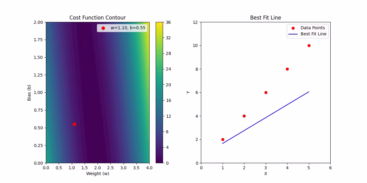
Line of Best Fit: What It Represents

What is the Line of Best Fit?

The line of best fit is the line that best represents the relationship between the input X (features) and the output Y (target). It minimizes the difference (error) between the observed data points and the predictions made by the linear regression model.

• Equation:
  The line is mathematically expressed as:

where:

• (fw,b( X)) is the predicted value of Y for input X.
• w determines the slope of the line.
• b shifts the line up or down.

Why "Best Fit"?

To identify the "best" line, we aim to minimize the errors between actual (Y) and predicted values (fw,b( X)) or Y.

• Residuals:
  The residual for each data point is:

Residuals represent the difference between observed and predicted values.

• Cost Function (Mean Squared Error):
  To quantify the error across all data points, we use:

Here:

• mmm is the number of data points.
• The 1/2m​ simplifies derivatives during gradient descent.

Mathematics Behind Linear Regression

Objective: Minimize the Cost Function

Our goal is to find the values of w and b that minimize J(w,b).

Gradient Descent: Optimizing w and b

Gradient descent is an iterative optimization algorithm used to minimize the cost function by updating the parameters www and b.

1. Initialization:some text
   • Start with initial values w=0, b=0 (or random values).
2. Update Rules: For each iteration:

Here:

α is the learning rate, controlling the step size.

Partial Derivatives of J(w,b):

Iterative Process:

• Update w and b using the gradients.
• Stop when the cost function converges (i.e., changes become negligible).

‍

‍

‍

Types of Linear Regression

Linear regression can be applied in different ways depending on the number of independent variables (predictors) and the complexity of the relationship between the variables. Here's an overview of the most common types of linear regression:

1. Simple Linear Regression

In simple linear regression, there is only one independent variable (predictor) and one dependent variable (target).

Equation:
            y=w⋅x+b

where x is the input feature, w is the weight (slope), and b is the bias (intercept).

It's useful when the relationship between the independent and dependent variables is straightforward and can be approximated by a straight line.

Example: 

Predicting a person’s salary based on years of experience. The more years of experience (x), the higher the salary (y).

2. Multiple Linear Regression

Multiple linear regression involves more than one independent variable (predictor). The goal is to model the relationship between the target variable and multiple predictors.

Equation:

           y=w1​⋅x1​+w2​⋅x2​+⋯+wn​⋅xn​+b

Where x1,x2,........, xn​ are the input features, w1,w2,....,wn ​are their respective weights, and b is the bias term.

This is useful when you have multiple factors that influence the outcome, and you want to predict the target based on those multiple factors.

Example:

Predicting a person’s salary based on multiple factors such as years of experience, education level, and number of certifications.

3. Polynomial Linear Regression

Polynomial regression is an extension of linear regression where the relationship between the independent and dependent variable is modeled as an nth degree polynomial.

Equation:

y=w0​+w1​⋅x+w2​⋅x2+w3​⋅x3+⋯+wn​⋅xn

where x is the independent variable and w0, w1,........., wn​ are the weights associated with 

When to Use Polynomial Regression:

• When there is a curvilinear (non-linear) relationship between the predictor and the target variable.
• For example, predicting the growth of a plant where the growth rate initially accelerates, then decelerates after reaching a peak.

Challenges:

• Overfitting: Higher-degree polynomials can easily overfit the data, especially when the data is noisy. This means the model might fit the data too well but fail to generalize to unseen data.
• Interpretability: Polynomial regression models become harder to interpret as the degree increases.

4. Ridge Regression (L2 Regularization)

Ridge regression is a variant of linear regression that introduces a penalty term to the cost function. This penalty term helps to regularize the model by shrinking the coefficients of less important features towards zero, which can prevent overfitting. This is particularly useful when the data has many features, or multicollinearity is present (when features are highly correlated).

Mathematics of Ridge Regression

In ridge regression, the cost function is modified by adding a penalty proportional to the sum of the squared values of the coefficients w. The modified cost function becomes:

‍

Where:

• Sum of Squared Errors is the usual loss function from linear regression.
• λ is a hyperparameter (regularization parameter) that controls the strength of the penalty. A higher λ will result in greater regularization (more shrinkage), while a smaller λ will result in less regularization.

Why Use Ridge Regression?

• Multicollinearity: When predictors are highly correlated, the coefficients in a simple linear regression model can become large and unstable. Ridge regression helps to control this instability.
• Overfitting Prevention: It prevents the model from fitting the noise in the training data by imposing a penalty on large coefficients.

Example:

Suppose you are predicting housing prices, and you have many features such as square footage, number of bedrooms, proximity to schools, etc. Some of these features may be highly correlated (e.g., square footage and number of rooms). In such cases, ridge regression can help ensure that the model doesn’t place too much importance on correlated features, making the model more stable.

5. Lasso Regression (L1 Regularization)

Lasso regression (Least Absolute Shrinkage and Selection Operator) is another variant of linear regression that uses L1 regularization. Unlike ridge regression, which penalizes the sum of squared coefficients, Lasso penalizes the sum of the absolute values of the coefficients. This results in some coefficients being exactly zero, effectively performing feature selection.

Mathematics of Lasso Regression

In Lasso regression, the cost function is modified by adding a penalty term proportional to the sum of the absolute values of the coefficients:

Where:

• λ controls the strength of the penalty. A higher λ\lambdaλ leads to more shrinkage, and more coefficients are set to zero.
• i=1n|wi| is the L1 penalty term.

Why Use Lasso Regression?

• Feature Selection: Lasso tends to drive some coefficients exactly to zero, which is useful for feature selection. This means it can help identify which features are most important in predicting the target.
• Overfitting Prevention: Like ridge regression, Lasso also prevents overfitting, but with the added advantage of sparse models (some coefficients becoming zero).

Example:

Imagine you are predicting customer churn using a set of features like age, income, subscription duration, customer satisfaction score, etc. Lasso regression can help identify which features are the most important, and it may shrink some of the unimportant features’ coefficients to zero.

‍

6. Elastic Net Regression

Elastic Net regression combines both Ridge and Lasso regularization techniques. It adds both L1 and L2 penalties to the cost function, which allows it to balance the benefits of both methods. Elastic Net is particularly useful when there are many correlated predictors.

Mathematics of Elastic Net Regression

The cost function for Elastic Net regression combines both the L1 and L2 penalties:

Where:

• λ1controls the L1 penalty (like in Lasso).
• λ2 controls the L2 penalty (like in Ridge).
• Elastic Net is particularly useful when the data contains highly correlated predictors and when we want a model that can both select relevant features (L1) and handle multicollinearity (L2).

Why Use Elastic Net?

• Combining Benefits of Lasso and Ridge: Elastic Net is a good option when you want the feature selection properties of Lasso and the stability of Ridge.
• When Features are Highly Correlated: It is especially effective when the number of predictors is greater than the number of observations, or when predictors are highly correlated.

Example:

Suppose you are modeling customer demand with features such as age, gender, income, product preferences, etc. If some of these features are highly correlated (e.g., income and spending), Elastic Net can help prevent overfitting and choose relevant predictors.

Evaluating Model Performance

After building a linear regression model (or any machine learning model), it's essential to evaluate its performance to ensure it is making accurate predictions. The quality of a model can be measured using various metrics that quantify how well it fits the data and how effectively it generalizes to unseen data.

Since we have already discussed various types of linear regression, including Ridge, Lasso, and Elastic Net, let’s dive into how we can evaluate the performance of these models.

1. Mean Absolute Error (MAE)

The Mean Absolute Error (MAE) measures the average of the absolute differences between predicted values and actual values. It gives us a sense of how far off the predictions are, on average, in terms of the original units of the target variable.

Where:

• yi is the actual value,
• ŷi​ is the predicted value, and
• n is the number of data points.

Advantages of MAE:

• MAE is easy to interpret because it uses the same units as the target variable.
• It is less sensitive to outliers compared to other metrics like MSE.

Limitations of MAE:

• MAE does not penalize larger errors as much as MSE, which can sometimes be a disadvantage in cases where large errors are more important.

2. Mean Squared Error (MSE)

The Mean Squared Error (MSE) measures the average of the squared differences between the predicted values and the actual values. Squaring the differences penalizes larger errors more heavily, making MSE sensitive to outliers.

Where:

• yi​ is the actual value,
• ŷi​ is the predicted value, and
• n is the number of data points.

Advantages of MSE:

• MSE is useful when larger errors are more costly because it penalizes them more severely.
• It is widely used in optimization algorithms such as gradient descent, as its derivative is easy to compute.

Limitations of MSE:

• MSE can be disproportionately influenced by outliers due to the squaring of errors.
• It does not provide an easily interpretable scale compared to MAE.

3. Root Mean Squared Error (RMSE)

The Root Mean Squared Error (RMSE) is simply the square root of the MSE, bringing the metric back to the same scale as the target variable. RMSE is sensitive to large errors, much like MSE, but it is more interpretable.

Advantages of RMSE:

• Like MSE, RMSE penalizes large errors and is widely used in machine learning.
• RMSE is easier to interpret than MSE, as it has the same units as the target variable.

Limitations of RMSE:

• RMSE is also highly sensitive to outliers, meaning a few large errors can greatly impact the value.

4. R-Squared (R²)

The R-squared (R²), also known as the coefficient of determination, measures the proportion of the variance in the dependent variable that is predictable from the independent variables. It provides insight into how well the model explains the variation in the data.

Where:

• yi is the actual value,
• ŷi is the predicted value, and
• y​ is the mean of the actual values.

Interpretation of R²:

• An R² value of 1 means the model perfectly explains the variance in the target variable.
• An R² value of 0 means the model does not explain any of the variance (i.e., a constant model).
• Negative R² values can occur if the model performs worse than a simple mean-based prediction.

Advantages of R²:

• R² is a standard metric in linear regression and provides a clear sense of how well the model fits the data.
• It is widely used for model comparison in regression tasks.

Limitations of R²:

• R² may not decrease if we add irrelevant features to the model, leading to overfitting.
• It can be misleading when comparing models with different numbers of predictors or when the data is not linear.

5. Adjusted R-Squared (Adjusted R²)

The Adjusted R-squared (Adjusted R²) is an adjusted version of R² that takes into account the number of predictors in the model. It adjusts for the fact that adding more variables to the model may artificially increase R², even if those variables don’t improve the model’s performance.

Where:

• n is the number of observations,
• p  is the number of predictors (features), and
• R2 is the standard R-squared.

‍

Advantages of Adjusted R²:

• Adjusted R² is particularly useful when comparing models with different numbers of features.
• It helps avoid overfitting by penalizing the inclusion of irrelevant predictors.

Limitations of Adjusted R²:

• It can be less interpretable than R², especially when comparing models with few predictors.
• It still doesn't address all issues of overfitting.

6. Cross-Validation

Cross-validation is a technique for assessing how the model will generalize to an independent dataset. It helps to identify overfitting by splitting the dataset into multiple subsets and training the model on each subset while evaluating it on the remaining data.

The most common type of cross-validation is k-fold cross-validation, where the data is divided into kkk subsets. The model is trained on k−1 subsets and evaluated on the remaining one, and this process is repeated for each subset.

Advantages of Cross-Validation:

• Provides a more reliable estimate of model performance than a simple train-test split.
• Helps prevent overfitting and ensures that the model generalizes well to new data.

Limitations of Cross-Validation:

• Can be computationally expensive, especially with large datasets or complex models.
• May not be suitable for time-series data, where future data points depend on past ones.

Choosing the Right Evaluation Metric

• For large datasets where large errors have a significant impact, RMSE is commonly used due to its ability to penalize larger errors more heavily.
• For simpler models, or when it’s important to treat all errors equally, MAE might be preferred.
• R-squared and Adjusted R-squared are useful when comparing multiple models to determine how well the predictors explain the variation in the target variable.
• Cross-validation is highly recommended when you want to evaluate the model’s generalizability.

‍

Evaluating the performance of a linear regression model (or any machine learning model) is essential to understand how well it is generalizing to new, unseen data. By using metrics such as MAE, MSE, RMSE, R², and Adjusted R², you can gain valuable insights into the accuracy of your model and its ability to make predictions.

Once you have trained and evaluated your model, the next step is to focus on model improvement (e.g., through regularization, feature engineering, or hyperparameter tuning), depending on the performance results.

Great! Let’s dive into Model Improvement Techniques. This section will focus on strategies to improve the performance of a linear regression model and make it more robust, accurate, and generalizable.

Model Improvement Techniques

Once you’ve built a basic linear regression model, the next step is to evaluate its performance and then improve it if necessary. Here are several techniques to improve your model:

1. Feature Engineering

Feature engineering is the process of using domain knowledge to create new features from the existing data. Better features often lead to better models, so it's crucial to explore your data and try to enhance it.

• Creating Interaction Terms: Sometimes, combining features can provide more informative predictors. For example, if you have two features like Height and Weight, their product (Height * Weight) might offer more predictive power.
  
  
• Polynomial Features: If your data isn’t well-represented by a linear model, consider adding polynomial features (e.g., x2x^2, x3x^3) to capture more complex relationships.
  
  
• Feature Scaling: In some cases, scaling your features so that they have the same range can improve the efficiency of your model, especially if you are using regularization techniques like Ridge or Lasso.
  
  

2. Regularization (Ridge, Lasso, and Elastic Net)

We already discussed Ridge and Lasso regression. Both methods help improve the model by reducing overfitting, which is common in models with too many features.

• Ridge Regression (L2 Regularization): Adds a penalty to the size of the coefficients, which helps reduce overfitting. Ridge is useful when dealing with many features that are not necessarily redundant but are highly correlated.
  
  
• Lasso Regression (L1 Regularization): Lasso can set some coefficients to zero, effectively performing feature selection. This can be helpful if you have many irrelevant features and want to eliminate them automatically.
  
  
• Elastic Net: A combination of L1 and L2 regularization, Elastic Net balances the benefits of both Ridge and Lasso regression. It's a good choice when you have a mix of useful and redundant features.
  
  

By tuning the regularization parameter (e.g., λ\lambda in Ridge or Lasso), you can control how much penalty is applied to the coefficients, finding the sweet spot between underfitting and overfitting.

3. Hyperparameter Tuning

Hyperparameters control the learning process of your model and can significantly affect its performance. For linear regression models, the most important hyperparameters typically relate to regularization strength (for Ridge, Lasso, and Elastic Net) and the learning rate for optimization techniques (e.g., if you're using gradient descent).

• Grid Search: This technique exhaustively tests a range of hyperparameters to find the best combination. For example, you might try different values of λ\lambda (regularization strength) in Ridge or Lasso.
  
  
• Random Search: Random search samples hyperparameters randomly from a predefined distribution. It can be more efficient than grid search in large search spaces.
  
  
• Cross-Validation: Use cross-validation in conjunction with hyperparameter tuning to get an unbiased estimate of the model's performance with different settings.
  
  

4. Cross-Validation

Cross-validation, particularly k-fold cross-validation, is a powerful technique to assess the model's generalization ability. It helps in selecting the model and its hyperparameters based on how well they perform on multiple train-test splits of the dataset.

• Stratified Cross-Validation: For classification problems where class imbalance exists, stratified k-fold ensures that each fold has the same proportion of classes, preventing model bias toward the majority class.
  
  
• Leave-One-Out Cross-Validation (LOO-CV): A special case of cross-validation where one data point is used for testing while the remaining data points are used for training. It can be computationally expensive but provides the most thorough assessment of model performance.
  
  

5. Removing Outliers

Outliers can distort the fit of a linear regression model, especially when using metrics like MSE, which heavily penalizes large errors. Detecting and removing outliers from the dataset can sometimes improve model performance.

• Box Plots and Scatter Plots: Use these visual tools to identify outliers.
• Z-Score or IQR: Statistical methods like Z-score (standard deviation) or Interquartile Range (IQR) can help in detecting outliers.

However, before removing outliers, ensure they aren’t important for the underlying problem. Sometimes, outliers carry valuable information.

6. Adding Interaction Terms

Sometimes, the relationship between the dependent and independent variables isn’t purely linear, but the interaction between two or more features might be. In this case, you can add interaction terms as additional features to capture these relationships.

For example, if you have features like X1 and X2, you might include an interaction term X1*X2 in the model.

7. Non-Linear Models

If the relationship between the dependent and independent variables is non-linear, linear regression may not be the best model. In such cases, you can explore non-linear models such as:

• Polynomial Regression: Fits a polynomial curve to the data, which allows for more flexibility than a straight line. This can capture nonlinear trends in the data.
  
  
• Decision Trees or Random Forests: If the relationship is more complex, tree-based models might be a better choice. These models are non-linear and handle interactions naturally.
  
  

8. Feature Selection

If you have many features, some of them might be irrelevant or redundant. Redundant or irrelevant features can lead to overfitting, slow model training, and increased computational costs.

Feature selection techniques help identify the most important features:

• Backward Elimination: Starts with all features and removes the least significant ones, one by one, based on a criterion (e.g., p-value).
• Forward Selection: Starts with no features and adds the most significant ones step by step.
• Recursive Feature Elimination (RFE): This method iteratively removes the least important features and builds the model on the remaining features.

9. Learning Curves

A learning curve plots the model's performance (e.g., training error or validation error) against the number of training examples. It provides insights into whether the model is underfitting or overfitting.

• Underfitting: If the model's training error is high, it indicates that it is not capturing the complexity of the data.
• Overfitting: If there is a large gap between training and validation errors, it suggests that the model is too complex and is memorizing the data.

Learning curves can guide decisions regarding model complexity and the need for more data or regularization.

10. Ensemble Methods

Sometimes, combining multiple models can lead to better performance than using a single model. Ensemble methods combine predictions from different models to create a stronger overall prediction.

• Bagging: It involves training multiple instances of the same model on different subsets of the data and averaging their predictions. Random Forest is an example.
• Boosting: A sequential ensemble method where each model corrects the errors made by the previous one. Examples include Gradient Boosting and AdaBoost.

Improving the performance of a linear regression model involves multiple steps, ranging from enhancing the features to using regularization techniques, hyperparameter tuning, cross-validation, and exploring non-linear models when necessary. Each of these steps can significantly contribute to creating a more accurate and robust model that generalizes well to new data.

The techniques discussed above are part of the iterative process of model improvement. You may need to revisit different steps (e.g., feature engineering, regularization) as you gain more insights into the problem and data. By constantly refining and testing your model, you can ensure better predictive performance and reliability.

Great! Let's move on to Practical Applications of Linear Regression. This section will focus on real-world problems where linear regression is commonly applied, helping you understand its practical utility in various industries.

Practical Applications of Linear Regression

Linear regression is one of the most widely used statistical techniques because it is simple, interpretable, and effective in many practical situations. Below are some of the real-world applications where linear regression plays a crucial role:

1. Predicting House Prices

In real estate, predicting the price of a house based on various features (such as size, number of bedrooms, location, etc.) is a classic example of linear regression. The model learns the relationship between these features and the house price, allowing for accurate predictions.

Example Features:

• Size of the house (in square feet)
• Number of bedrooms and bathrooms
• Location (e.g., zip code, neighborhood)
• Age of the house
• Proximity to public transport

By applying linear regression, we can predict the price of a house, which helps both sellers and buyers make informed decisions.

2. Sales Forecasting

Companies use linear regression to forecast sales based on historical data and various factors, such as marketing spend, seasonal effects, and economic conditions. This helps businesses plan production schedules, stock inventory, and allocate marketing budgets.

Example Features:

• Advertising budget
• Time of year (seasonality)
• Market conditions
• Previous sales data

By predicting future sales, businesses can optimize their operations and improve profitability.

3. Stock Market Prediction

Linear regression is also used to predict stock prices and returns. While stock prices are influenced by a variety of factors (e.g., market sentiment, company performance, economic indicators), linear regression can help model relationships between these factors and stock price movements.

Example Features:

• Historical stock prices
• Trading volume
• Economic indicators (e.g., inflation rate, interest rates)
• Company financial performance (e.g., revenue, profits)

Though stock prices are often volatile, linear regression can be helpful for analyzing trends and making short-term predictions.

4. Healthcare: Predicting Disease Progression

In healthcare, linear regression is used to model the progression of diseases or to predict patient outcomes based on clinical data. For instance, it can predict the progression of diabetes or the likelihood of recovery after surgery based on various medical parameters.

Example Features:

• Age
• Blood pressure
• Cholesterol levels
• Family medical history
• Lifestyle factors (e.g., smoking, exercise)

These predictions can help healthcare providers make better decisions and personalize treatment plans for patients.

‍

5. Marketing and Customer Insights

Marketing teams use linear regression to analyze customer behavior and make data-driven decisions. By understanding the relationship between customer attributes (such as demographics) and purchasing decisions, companies can improve their marketing strategies and increase conversion rates.

Example Features:

• Customer age, gender, and income
• Product features (e.g., price, quality)
• Marketing campaign features (e.g., discounts, promotions)
• Past purchasing behavior

Linear regression helps companies understand what factors drive consumer behavior and optimize their marketing efforts accordingly.

6. Climate and Environmental Studies

Linear regression is used to study climate change and predict future environmental conditions. For example, researchers can model the relationship between atmospheric CO2 levels and temperature increases, which helps in forecasting the future impacts of climate change.

Example Features:

• Atmospheric CO2 concentration
• Temperature records
• Seasonal variations
• Other greenhouse gases (e.g., methane)

Understanding these relationships can guide policy decisions and strategies for combating climate change.

7. Manufacturing and Quality Control

In manufacturing, linear regression is used to model and predict product quality based on production parameters. This allows companies to identify factors that contribute to defects or inefficiencies in the production process.

Example Features:

• Temperature during manufacturing
• Pressure applied in machinery
• Raw material quality
• Machine settings (e.g., speed, torque)

By identifying key factors affecting product quality, manufacturers can optimize processes and reduce defects.

8. Sports Analytics

Sports teams and analysts use linear regression to predict player performance and team success. For example, they might predict a player’s performance based on their historical data or the team’s performance based on past games.

Example Features:

• Player statistics (e.g., goals, assists, shooting accuracy)
• Training data (e.g., workout intensity)
• Opponent strength
• Team dynamics (e.g., number of injuries, team morale)

By predicting performance, coaches can make better decisions on team strategy and player selection.

9. Education: Student Performance Prediction

Educational institutions use linear regression to predict student performance based on various factors such as prior academic performance, attendance, and socio-economic background.

Example Features:

• Previous grades and test scores
• Attendance rates
• Parental involvement
• School resources

This helps in identifying students who may need additional support or resources, improving educational outcomes.

10. Transportation and Traffic Prediction

In transportation planning, linear regression is used to predict traffic patterns and optimize routes. By modeling the relationship between traffic flow and factors like time of day, weather, and construction, cities can better plan for traffic management.

Example Features:

• Time of day
• Weather conditions (e.g., rain, snow)
• Roadwork or accidents
• Population density

This helps reduce traffic congestion and improve transportation efficiency.

Linear regression is a versatile tool used across various industries for predicting outcomes and making data-driven decisions. Whether you are predicting house prices, sales, disease progression, or environmental changes, linear regression provides a simple yet powerful way to model relationships between variables and make informed predictions.

By applying the concepts of feature selection, regularization, and model evaluation, you can improve your linear regression model’s accuracy and ensure it performs well in real-world applications.

‍

Common Challenges in Linear Regression

While linear regression is a powerful and straightforward tool, it comes with several challenges that can affect the quality of the model’s predictions. Understanding these challenges and knowing how to mitigate them is crucial for building accurate and reliable models.

Here are some of the most common challenges you might encounter when working with linear regression:

1. Overfitting

Overfitting occurs when the model learns the details and noise in the training data to such an extent that it negatively impacts the performance of the model on new, unseen data. This happens when the model becomes too complex, often due to including too many features or polynomial terms.

Signs of Overfitting:

• The model performs exceptionally well on the training data but poorly on validation or test data.
• The error metrics (e.g., MSE or RMSE) are significantly higher on the test data than on the training data.

How to Address Overfitting:

• Regularization (e.g., Lasso, Ridge) can be used to penalize large coefficients and prevent the model from becoming too complex.
• Cross-validation helps identify overfitting by evaluating the model on different subsets of the data.
• Reducing the number of features can also help simplify the model and prevent overfitting.

2. Underfitting

On the opposite side of overfitting, underfitting occurs when the model is too simple to capture the underlying patterns in the data. This usually happens when the model has too few features or when the relationship between the features and target variable is not truly linear.

Signs of Underfitting:

• The model performs poorly both on the training data and test data.
• The model fails to capture the trends in the data and results in high error values.

How to Address Underfitting:

• Try adding more features or using higher-degree polynomials if appropriate.
• Consider using more complex models (e.g., decision trees, support vector machines) if the relationship is not linear.

3. Multicollinearity

Multicollinearity occurs when two or more predictors (independent variables) in the model are highly correlated. This can cause instability in the model’s coefficient estimates, leading to unreliable predictions. In such cases, small changes in the data can result in large changes in the model's predictions.

Signs of Multicollinearity:

• The model’s coefficients have very high standard errors.
• Some coefficients may appear to be insignificant, even though they should be significant.

How to Address Multicollinearity:

• Remove highly correlated features: Use correlation analysis or a variance inflation factor (VIF) to identify and remove highly correlated predictors.
• Principal Component Analysis (PCA): PCA can be used to reduce the dimensionality of the data and eliminate multicollinearity by transforming the features into orthogonal components.
• Regularization (e.g., Ridge regression) helps to mitigate the effects of multicollinearity by shrinking the coefficients.

4. Homoscedasticity vs. Heteroscedasticity

Homoscedasticity means that the variance of the errors (residuals) is constant across all levels of the independent variable(s). On the other hand, heteroscedasticity occurs when the variance of the residuals is not constant and tends to increase or decrease with the value of the independent variable(s).

Signs of Heteroscedasticity:

• The residual plot shows a pattern, such as a funnel shape, indicating that the error variance is changing as the value of the predictors changes.

How to Address Heteroscedasticity:

• Transform the dependent variable: Apply a transformation like logarithmic or square root to stabilize the variance.
• Weighted least squares regression: In cases where variance is not constant, weighted least squares can be used to give more weight to data points with less variance.

5. Outliers and Influential Data Points

Outliers are data points that deviate significantly from the rest of the data. They can have a disproportionate impact on the model’s performance, especially in linear regression, where the objective is to minimize the squared error.

How to Identify Outliers:

• Visual methods: Use scatter plots, box plots, or residual plots to detect unusual points that are far from the general trend.
• Statistical methods: Calculate z-scores or use the Interquartile Range (IQR) method to identify outliers.

How to Handle Outliers:

• Remove or adjust outliers: If an outlier is due to a data error, you can remove it. However, if the outlier is valid, you may want to adjust it or transform the data.
• Use robust regression techniques: Techniques like Huber regression can be used to reduce the influence of outliers.

6. Non-Linearity

Linear regression assumes that the relationship between the independent variables and the target variable is linear. However, real-world data may not always follow a linear relationship. In such cases, applying linear regression may lead to poor model performance.

Signs of Non-Linearity:

• A scatter plot of the data shows a non-linear trend (e.g., a curve or other patterns).
• The residual plot shows patterns or structures instead of random noise.

How to Address Non-Linearity:

• Polynomial regression: Introduce polynomial terms (e.g., x2x^2, x3x^3) to capture non-linear relationships.
• Non-linear regression models: Consider using other models, such as decision trees or neural networks, that can handle complex non-linear relationships.
• Feature engineering: Create new features that may better capture the underlying patterns in the data.

7. Assumptions Violations

Linear regression makes several assumptions about the data. Violating these assumptions can lead to inaccurate models. The key assumptions of linear regression are:

1. Linearity: The relationship between the dependent and independent variables is linear.
2. Independence: The residuals (errors) are independent of each other.
3. Normality: The residuals should be normally distributed.
4. Homoscedasticity: The variance of the errors should be constant across all values of the independent variables.

How to Check Assumptions:

• Residual plots: Check for patterns in the residuals to assess linearity, independence, and homoscedasticity.
• Q-Q plot: A quantile-quantile plot can help you check for the normality of residuals.

How to Address Assumptions Violations:

• Transform the data: Apply transformations like logarithms to make the data more linear or make the residuals more homoscedastic.
• Consider other models: If the assumptions are severely violated, consider using non-linear regression or robust regression models.

Also Read: The Role of Machine Learning Repositories in Providing Valuable Datasets for Machine Learning

While linear regression is a powerful and interpretable tool, it’s essential to be aware of the common challenges that can affect its performance. By understanding issues such as overfitting, multicollinearity, heteroscedasticity, and non-linearity, you can take steps to improve the model’s robustness and predictive power. Regularization techniques like Ridge and Lasso, along with model evaluation metrics, can help you build better models that generalize well to unseen data.

Conclusion

Linear regression, though simple, is a foundational technique in machine learning and statistical modeling. It provides a clear understanding of the relationship between variables and serves as a stepping stone to more complex algorithms. By mastering its concepts—such as the linear regression equation, the importance of the cost function, gradient descent, and the various types like polynomial regression, ridge, and lasso regression—you gain a solid base for predictive modeling and data analysis.

Understanding the assumptions of linear regression and evaluating the model’s performance ensures its correct application. While challenges like multicollinearity or outliers might arise, addressing them appropriately can lead to robust and interpretable models.

Whether you're predicting trends in finance, understanding customer behavior in marketing, or making forecasts in healthcare, linear regression remains a powerful and versatile tool. With this guide, you’re now equipped with the knowledge to confidently apply linear regression and build upon this skill for more advanced modeling techniques.

‍